Measuring Phase in Software - Phase Noise, IQ Data and the Analytic Signal

Motivation

Often in my research I need to measure the phase of a signal. This signal will commonly be a radio-frequency (RF) tone, described as a time varying voltage $V(t)$,

\[V(t)=A\cos(2\pi f t +\alpha(t)).\]

Here, $A$ is the amplitude of the tone, $f$ is the frequency of the tone, $t$ is the measurement time, and $\alpha(t)$ is some arbitrary phase (which may depend on time). In this post, I want to run through some tools I’ve found useful for measuring $\alpha(t)$. The end-goal for this series of blog posts will be a software phase-locked loop (PLL). In short, this is a control system that actively tracks the phase of a tone. The end-goal for this series will be implementing an all-digital PLL inside the field-programmable gate array (FPGA) of a Pluto software-defined radio (SDR). Rather than jumping straight to the FPGA, I want to take the time to describe some important signal processing theory. This can all be done in software, which is a bit easier to work with.

Overview

Prior to reading this post, I highly recommend going through PySDR: A Guide to SDR and DSP using Python [1]. It goes into great detail on in-phase and quadrature (IQ) sampling, and signal processing on IQ samples. I’m also going to assume familiarity with Python, Fourier transforms, Z-transforms, power spectrums and power spectral densities.

In this post, I want to cover the following theory:

1. How we can model noise in $V(t)$
2. Phasors, and what measuring phase actually mean
3. The Hilbert transform and its relationship to IQ data

I also want to show how additive noise can contribute to phase measurements. After getting the theory out of the way, I’ll start using Python to generate data.

There’s a bit to cover. We could just jump straight to code for a PLL, and of course you’re welcome to do so (skip to the end). However, if you take the time to understand the tools I present here, you will be able to simulate and understand a multitude of experimental conditions.

Modelling Noise

There’s two classes of noise that we need to consider. Firstly, there’s additive noise. Additive noise is what we usually think about when we hear noise in a signal processing context. Simply put, it’s random variations added on to the voltage of our signal. I like to model it as $\bar{A}(t)$, with our measured voltage being,

\[V(t)=A\cos(2\pi f t +\alpha(t))+\bar{A}(t).\]

Additive noise is often associated with electronic noise. I won’t limit this generalisation to additive white Gaussian noise, but, more often than not, most additive noise sources I work with are white (e.g. shot noise on a photodetector).

Secondly, there’s phase noise. I think of this as random variations in the phase delay of, or arrival time of, our signal. There are a great deal of phase noise sources. I recommend taking a quick read of Enrico’s Chart for Phase Noise and Two-Sample Variances [2]. We can accommodate for phase noise fluctuations, $\bar{\epsilon}(t)$, in our voltage model as,

\[V(t)=A\cos(2\pi f t +\alpha(t)+\bar{\epsilon}(t))+\bar{A}(t).\]

It can be helpful to instead consider a phasor model of $V(t)$. I’ve drawn such a model in Figure. 1.

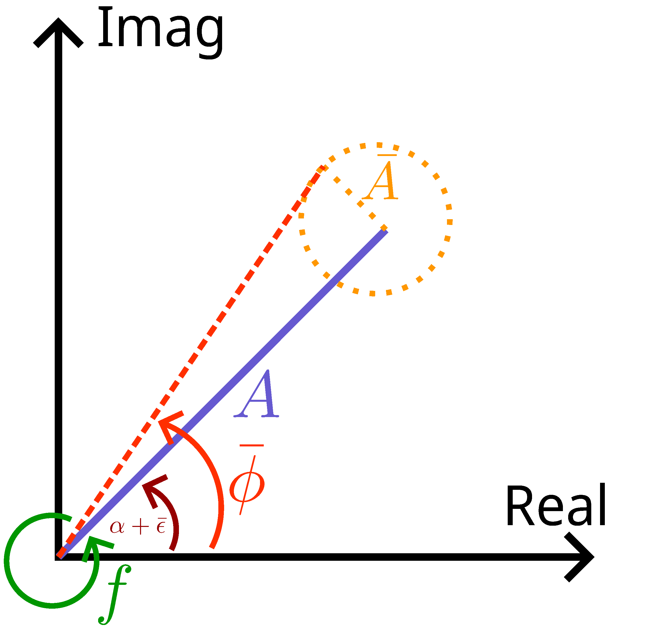
Figure 1: Phasor diagram of the voltage model. $f$, the rate at which our phasor spins; $\bar{\phi}$ the phase that our PLL will measure; $A$, the amplitude (magnitude) of the measurement signal; $\bar{A}$, the additive amplitude noise in the measurement signal; $\bar{\epsilon}$, the phase noise of the signal.

Our phasor model is a complex exponential,

\[\pmb{V}=\bar{A}e^{j{\bar{\phi}}}.\]

Here I’ve lumped the phase and amplitude terms into $\bar{A}$ and $\bar{\phi}$. We should note that this is no longer a voltage, rather it is a model for what the phase and amplitude of our signal are doing at any given time. The phasor model will hopefully make a lot more sense when I introduce the Hilbert transform. Visually, the phasor diagram tells us a few things.

1. The phasor is rotating around the complex plane at a rate of $f$ Hz.
2. If we were to ‘subtract’ the rotating component of the phasor, we’re left with a point on the complex plane that is, hopefully, slowly moving. This is the purple line. The phase we care about, $\alpha(t)$, is the angle of this purple line.
3. Random phase perturbations $\bar{\epsilon}$ cause the angle of the purple line (phasor) to fluctuate.
4. Amplitude fluctuations $\bar{A}$, couple into both the real and imaginary component of the phasor. This results in a circle of uncertainty around the phasor’s point on the complex plane (orange circle).
5. The phase that we will measure, $\bar{\phi}$, is the combined result of both the additive and phase noise. The measured phase is the angle of the dashed red line.

Conceptually, these are the most crucial elements to understanding how we can measure the phase of our signal. To get a meaningful measurement, we need the ability to ‘subtract’ away the rotating component of the phasor. More intuitively, and practically, we can think of this as phase comparison. Consider if we had two rotating phasors,

\[\pmb{V_1}=A_1e^{j{\phi_1}},\] \[\pmb{V_2}=A_1e^{j{\phi_2}},\] \[\phi_1=2\pi f t,\] \[\phi_2=2\pi f t + \alpha.\]

It is practically easier to compare the phase of two signals. We will call $\pmb{V_1}$ our local oscillator, which provides a stable phase reference to compare $\pmb{V_2}$ to. We can readily extract the phase of our signal as,

\[\alpha=\arg(\pmb{V_2V_1^*})=\arg(A_1A_2e^{j\alpha}).\]

The phasor model also tells us how noise will couple into our measurement. If we were to look at $\arg(\pmb{V_2V_1^*})$ in practice, we would not obtain $\alpha$. Rather we would obtain a combination of the phase we care about, $\alpha$, the phase noise, $\bar{\epsilon}$, and the additive noise, $\bar{A}$. To further describe how additive noise couples into our measurement, I would like to introduce the Hilbert transform and the Analytic signal.

A Brief Review of IQ Sampling

I think it’s most useful to mention IQ sampling here. Rather than sampling $V(t)$ directly, we can sample its I and Q components. Again, I highly recommend reading PySDR [1] for a more thorough description. For a signal $x(t)=A\cos(2\pi f t-\phi)$, we can, through some trigonometry, express it as,

\[x(t)=I\cos(2\pi f t)+Q\sin(2\pi f t),\] \[I=A\cos(\phi),\] \[Q=A\sin(\phi).\]

Most SDRs will sample I and Q, some sample $V(t)$ directly. Soon, I will talk about going back and forth between the two. In Physics and Engineering, we like to use complex exponentials. They’re slightly easier to work with mathematically, and, arguably also easier to work with numerically. What’s nice about IQ data, is that it naturally describes a phasor. The magnitude of the IQ phasor, $A$, is obtained from,

\[A=\sqrt{I^2+Q^2},\]

and the phase, $\phi$,

\[\phi=\tan^{-1}(Q/I).\]

Thus, we can describe our IQ data as a phasor, $\pmb X$,

\[\pmb{X}=I+jQ,\] \[A=|I+jQ|,\] \[\phi=\angle(I+jQ).\]

What’s nice about IQ data is that the rotating part of the phasor, herein called the carrier, is subtracted off for us in the analogue front end of the receiver. An important clarification is that the IQ phasor $\pmb X$ is used as it makes our life easy. We can readily analyse imaginary data in software. We can take its FFT to visualise what makes up our signal. We can frequency up-shift and down-shift simply by mixing the IQ data with a complex exponential. We can also readily extract phase and amplitude by taking the magnitude or argument of our IQ samples. It’s important to remember that our data, $\pmb X=I+jQ$, represents the two independent quadratures of a physical signal, related back to $x(t)$ via,

\[x(t)=I\cos(2\pi f t)+Q\sin(2\pi f t).\]

Analytic Signals

With a good understanding of IQ sampling and the IQ phasor, we can introduce what’s called an analytic signal. A good place to look for information is the SciPy reference [3] and [4]. To best understand this, let’s look at a very useful analytic signal, the complex exponential,

\[\hat{u}(t)=Ae^{j\phi(t)}=A\cos(\phi(t))+jA\sin{\phi(t)}.\]

The key properties of an analytic signal are:

• The imaginary component, $\sin(\phi)$ in this case, is the real component, $\cos(\phi)$ here, shifted by $90^\circ$ degrees.
• The analytic signal, $e^{j\phi}$ here, has no negative frequency components. This can readily be verified by adding the fourier transforms of $\cos(\phi)$ and $j\sin(\phi)$.
• The imaginary component, $\sin(\phi)$, does not tell us anything new about our real signal $\cos(\theta)$.
  • Our original, real signal, is $\mathcal{Re}\{\hat u (t)\}$.

The reason we would use the analytic signal is that we can obtain the phase and amplitude quite easily with,

\[A=|\hat{u}(t)|,\] \[\phi(t)=\angle \hat{u}(t).\]

The analytic signal is a generalisation of the phasor. A phasor typically has no time dependence. To include a time dependence in the phasor model, is to make it an analytic signal. The reason I introduce it, is because there’s a useful tool called the Hilbert transform that can be used to generate the analytic signal from a real valued signal.

We can construct an analytic signal with,

\[\hat{u}(t)=x(t)+j\mathcal{H}\{x(t)\},\]

where $\mathcal{H}\{ \dots \}$ denotes the Hilbert transform. The Hilbert transform is, in and of itself, an integral transform. However, we can opt to relate it to the Fourier transform of $x(t)$. Essentially, the Hilbert transform phase shifts the signal $x(t)$. But, it actually applies a different phase shift to the positive and negative frequencies in the signal. The Fourier transform of $\mathcal{H}\{x(t)\}$, is,

\[\DeclareMathOperator{\sign}{sign}\mathcal{F}\{\mathcal{H}\{x\}\}=-j\sign(f)\mathcal{F}(x).\]

That is, the Hilbert transform rotates positive frequencies by $-90^\circ$ degrees, and negative frequencies by $+90^\circ$ degrees. Computationally, this is the easiest way to perform the Hilbert transform. You can take its FFT, and mix the positive frequency components by $-j$, and the negative frequency components by $+j$. Alternatively, you can take the FFT, zero out the negative frequencies, and double the positive frequencies. The inverse FFT would then provide the analytic signal directly.

The reason we would do this, is again convenience. It’s easier to determine the amplitude and phase of the analytic signal, than it is to extract it from the real valued signal. Complex numbers make things easier.

If we consider our original voltage model $V(t)=A\cos(2\pi f t + \alpha(t)+\bar{\epsilon}(t))+\bar{A}(t)$, we can readily construct its analytic signal (its phasor! shown in Figure 1) as,

\[\mathcal{H}\{V(t)\}=A\sin(2\pi f t+\alpha(t)+\bar\epsilon(t))+\mathcal{H}\{\bar{A}(t)\},\] \[\hat{u}(t)=A\cos(2\pi f t + \alpha(t)+\bar{\epsilon}(t))+\bar{A}(t) + j[A\sin(2\pi f t+\alpha(t)+\bar\epsilon(t))+\mathcal{H}\{\bar{A}(t)\}].\]

I like this approach, as it readily highlights that the additive noise will couple into both the imaginary and real component of our phasor model. That is, our phasor is corrupted by $\bar A(t)+j\mathcal{H}\{\bar A(t) \}$. This will help us model the impact of additive noise on our phase measurement. Before we do some fun math, a word of caution. It’s very easy to fall into the trap of thinking that IQ data and the analytic signal tell us the same thing (I’ve fallen into it myself). However, in general, they are different. The key distinction stems from a fundamental property of the analytic signal – the imaginary component does not tell us anything new about our signal, it’s dependent on the real signal we care about via the Hilbert transform. For IQ data however, we are looking at two independent quadratures, we cannot discern one from the other. Regardless, the analytic signal and IQ data that we would measure can be related to each other.

Here are some useful properties, derived using the analytic signal (hidden for clarity), that will be useful for our signal processing:

---

Property 1: Relationship with $x(t)=I\cos(2\pi f t)+Q\sin(2\pi f t)$

The IQ components of our voltage $V(t)$, can be related to the analytic signal via,

\[I=\mathcal{Re}\{\hat{u}(t)e^{-j2\pi f t}\},\]

and,

\[Q=-\mathcal{Im}\{\hat{u}(t)e^{-j2\pi f t}\}.\]

Here, the analytic signal is down-converted by mixing with the carrier $e^{-j2\pi f t}$. This is useful if you want to generate IQ data from a simulated real signal.

Click to expand

Consider a general signal to be transmitted, $$ x(t)=A\cos(2\pi f t - \phi)$$ It can be expressed as, $$ x(t)=I\cos(2\pi f t)+Q\sin(2\pi f t)$$ $$I=A\cos(\phi)$$ $$Q=A\sin(\phi)$$ The analytical signal is provided by, $$\hat{u}(t)=A\cos(2\pi f t - \phi)+j\mathcal{H}\{x(t)\}=A\cos(2\pi f t - \phi) + jA\sin(2\pi f t-\phi)=Ae^{j(2\pi f t-\phi)}$$ Let's separate the analytical signal into, $$ \hat{u}(t)=Ae^{-j\phi}e^{j2\pi f t}$$ We can also take $Ae^{-j\phi}=I_u+jQ_u$, $$ \hat{u}(t)=(I_u+jQ_u)e^{j2\pi f t}$$ Now, recall that $x(t)=\mathcal{Re}\{\hat{u}(t)\}$, $$ \hat{u}(t)=(I_u+jQ_u)e^{j2\pi f t}=(I_u+jQ_u)(\cos(2\pi f t)+j\sin(2\pi f t))=(I_u\cos(2\pi f t)-Q_u\sin(2\pi f t))+j(\dots)$$ From which we find that, $$x(t)=I_u\cos(2\pi f t)-Q_u\sin(2\pi f t)$$ This tells us that the conventional IQ data approach isn't quite consistent. From comparison with, $$x(t)=I\cos(2\pi f t)+Q\sin(2\pi f t),$$ we see that $I_u=I$ and $Q_u=-Q$. In other words, to get IQ data, we actually want the conjugate of the down shifted analytical signal $(\hat{u}e^{-j2\pi f t})^*$.

---

Property 2.1: Arbitrary Phase Modulation

We can generate a signal with arbitrary phase modulation , $\phi(t)$, by first generating the IQ samples, \(\pmb X = e^{j\phi(t)}=I+jQ.\) We then have two equivalent options of converting this to a real signal:

\[x(t)=I\cos(2\pi f t)+Q\sin(2\pi f t),\] \[x(t)=\mathcal{Re}\{\pmb X^* e^{j2\pi f t}\}.\]

Click to expand

We can verify $$x(t)=\mathcal{Re}\{\pmb X^* e^{j2\pi f t}\}$$ by direct evaluation. $$x(t)=\mathcal{Re}\{\pmb X^* e^{j2\pi f t}\} = \mathcal{Re} \{ (I-jQ)(\cos(2\pi f t) + j\sin(2\pi f t))\}$$ $$=\mathcal{Re}\{I\cos(2\pi f t)-j^2Q\sin(2\pi f t) + j(\dots) \}= I\cos(2\pi f t)+Q\sin(2\pi f t)$$

---

Property 2.2: Arbitrary Amplitude Modulation

We can generate a signal with arbitrary amplitude modulate, $A(t)$, by generating IQ samples,

\[\pmb X = A(t)e^{j\phi(t)}.\]

If we want to instead model an additive signal (or additive noise), $\bar{A}(t)$,

\[\pmb X =Ae^{j\phi(t)}+\bar{A}(t) - j\mathcal{H}\{\bar A (t)\}.\]

For this equation to make sense, $S_{\bar A}(f)$ should be defined from 0Hz to the sample rate $f_s$. The PSD would then be shifted up to the carrier when transmitting.

Click to expand

Consider the signal, $$ x(t)=A\cos(2\pi f t-\phi)+\bar{A}(t)$$ The analytical signal is, $$ \hat{u}(t)=(I_u+jQ_u)e^{j2\pi f t}+\bar{A}(t)+j\mathcal{H}\{\bar{A}\}$$ We can down convert this to figure out I and Q, $$\hat{u}(t)e^{-j2\pi f t}=I_u+jQ_u+(\bar{A}(t)+j\mathcal{H}\{\bar{A}\})(\cos(2\pi f t)-j\sin(2\pi f t))$$ $$ = [I_u + \bar{A}(t)\cos(2\pi f t)+\mathcal{H}\{\bar{A}\}\sin(2\pi f t)] + j[Q_u+\mathcal{H}\{\bar{A}\}\cos(2\pi f t)-\bar{A}\sin(2\pi f t)]$$ And from property 1, $$I=I_u + \bar{A}(t)\cos(2\pi f t)+\mathcal{H}\{\bar{A}\}\sin(2\pi f t)$$ $$Q=-(Q_u+\mathcal{H}\{\bar{A}\}\cos(2\pi f t)-\bar{A}\sin(2\pi f t))$$ Intuitively, our measurement will see additive noise around the carrier. In the IQ sampling process, the additive noise is frequency shifted down to 0Hz. This is why there are $\cos(2\pi f t)$ and $\sin(2\pi f t)$ terms. However, if we're directly generating noise from 0Hz to $f_s/2$, we can ignore the down-conversion process (it is implicitly assumed). This provides, $$I=I_u + \bar{A}(t)$$ $$Q=-(Q_u+\mathcal{H}\{\bar{A}\})$$ From which it is clear that, $$\pmb X =I+jQ=Ae^{j\phi(t)}+\bar{A}(t) - j\mathcal{H}\{\bar A (t)\}.$$

---

Property 3: Additive to Phase Noise Conversion

For an additive noise source with power spectral density (PSD) $S_\bar A(f)$, it is seen in our measurement as phase noise with a PSD $S_{\phi,\bar A}(f)$, given by,

\[S_{\phi, \bar A}(f)=\frac{2}{A^2}S_\bar A(f),\]

for signal amplitude $A$. This essentially tells us how our signal-to-noise (SNR) ratio limits our measurement. As our signal decreases, we see more additive noise in our phase measurement. This is a very important result!

Click to expand

A simplified model of the noise sources is given by: $$v(t)=A\cos(\omega t + \alpha(t) + \bar{\epsilon}(t)) + \bar{A}(t)$$ where $v(t)$ is the voltage of the signal input to our phase measurement device, $A$ is the amplitude of the signal, $\omega$ is the frequency of the signal, $\alpha$ is the deterministic phase of the signal we want to measure, $\bar{\epsilon}(t)$ is the phase noise, and $\bar{A}(t)$ is the amplitude noise. We can usually lump the phase we're interested in measuring, and its noise together. A PLL will be used to measure the phase of the signal. For the following, it is useful to think of the PLL as a device that outputs the phase $\phi(t)$, where, $$ \phi(t) = \alpha(t) + \bar{\epsilon}(t) + k \bar{A}(t). $$ Here, $\phi(t)$ is the total phase of the signal, $\alpha(t)$ is the signal we want to measure, $\bar\epsilon$ is the phase noise, and $k\bar{A}(t)$ is the amplitude noise. Here, $k$, is just to show that the amplitude noise couples into our measurement. We will work out very shortly how it does so. To avoid confusion, the phasor model can be separated into its time varying component and its phase component (ignoring additive noise): $$ v(t) = \mathcal{Re}\{Ae^{j\omega t}e^{j\phi}\}$$ and the ideal PLL measurement will be given by: $$ v(t) = \text{Arg}(Ae^{j\omega t}e^{j\phi}\times e^{-j\omega t})=\phi$$ There are a few ways to figure out how $\bar A$ will couple into the phase measurement from the PLL. I'm going to run through a derivation that uses the Hilbert transform, as it is essentially a mathematical description of the phasor diagram above. The goal is to find how the noise output, $S_{PLL}(f)$, depends on the phase noise $S_{\bar\phi}(f)$ and the additive noise $S_{\bar A}(f)$, where $S(f)$ is the noise power spectral density. While crude, this derivation will use: $$S(f)=\frac{1}{\text{RBW}}|\mathcal{F}(v(t))|^2$$ where $\mathcal{F}$ is the Fourier transform, $v(t)$ is the signal of interest and $\text{RBW}$ is the resolution bandwidth of our FFT. I'm mixing up continuous and discrete here, but it helps get the end result. Another approach can be found in [5]. As we're looking at how noise couples in to phase, we will ignore $\alpha(t)$. Starting with, $$v(t) = A \cos(\omega t + \bar{\epsilon}(t))+\bar{A}(t)$$ Take the Hilbert transform, $$\mathscr{H}\{v(t)\}=A\sin(\omega t + \bar{\epsilon}(t))+\mathscr{H}\{\bar{A}(t)\}$$ Form the analytic signal, $$u(t) = A \cos(\omega t + \bar{\epsilon}(t))+\bar{A}(t) + j[A\sin(\omega t + \bar{\epsilon}(t))+\mathscr{H}\{\bar{A}(t)\}]$$ The instantaneous phase $\bar{\phi}(t)$ is given by the argument of this analytic signal (which is the phase of the phasor drawn in Figure 1), $$\bar{\phi}(t) = \tan^{-1} [\frac{A\sin(\omega t + \bar{\epsilon}(t))+\mathscr{H}\{\bar{A}(t)\}}{A \cos(\omega t + \bar{\epsilon}(t))+\bar{A}(t)}]$$ For small $x,y$ it can be shown using a taylor expansion of $x$ and $y$ that, $$\tan^{-1}[\frac{\sin(\alpha)+x}{\cos(\alpha)+y}]\approx \alpha + x \cos(\alpha) - y \sin(\alpha)$$ from which it follows for small noise fluctuations $\bar{A}(t)$ that, $$\bar{\phi}(t) = \omega t + \bar{\epsilon}(t) + \frac{\mathscr{H}\{\bar{A}(t)\}}{A}\cos(\omega_i t + \bar{\epsilon}(t)) - \frac{\bar{A}(t)}{A}\sin(\omega_i t + \bar{\epsilon}(t))$$ We can remove the $\omega t$ component, leaving, $$\begin{aligned} \bar{\phi(t)}=\bar{\epsilon}(t)+\frac{\mathscr{H}\{\bar{A}(t)\}}{A}\cos(\omega t + &\bar{\epsilon}(t)) - \frac{\bar{A}(t)}{A}\sin(\omega t + \bar{\epsilon}(t))\\ \bar{\phi(t)} &= \bar{\epsilon}(t)+ A'(t) \end{aligned}$$ From this it is clear that, $$\begin{aligned} S_{\phi,\bar\epsilon}(f)=S_{\bar\epsilon}(f) \end{aligned}$$ which is expected. It is a bit more involved to work out the contribution from the additive noise. Let's just consider the additive noise now, $$ \bar{\phi(t)}=\frac{\mathscr{H}\{\bar{A}(t)\}}{A}\cos(\omega t + \bar{\epsilon}(t)) - \frac{\bar{A}(t)}{A}\sin(\omega t + \bar{\epsilon}(t)) $$ Using the property of the Hilbert transform $\mathcal{F}(\mathcal{H}(x(t)))=-j \mathcal{F}(x(t))$, we can obtain, $$ \mathcal{F}(\bar{\phi}(t)) = \mathcal{F}\{\frac{\mathcal{H}\{\bar{A}(t)\}}{A}\cos(\omega t + \bar{\epsilon}(t))\} + \mathcal{F}\{-\frac{\bar{A}(t)}{A}\sin(\omega t + \bar{\epsilon}(t))\} $$ To avoid confusion with the Fourier transform, I will take $\omega=2\pi f_c$, where $f_c$ is the carrier. I will also ignore $\bar\epsilon(t)$ inside the $\sin$ and $\cos$ terms. Using the convolution property of the Fourier transform, $$ \mathcal{F}(\bar{\phi}(t)) = \mathcal{F}\{\frac{\mathcal{H}\{\bar{A}(t)\}}{A}\} \ast \mathcal{F}\{\cos(2\pi f_c t + \bar{\epsilon}(t))\} + \mathcal{F}\{-\frac{\bar{A}(t)}{A}\} \ast \mathcal{F}\{\sin(2\pi f_c t + \bar{\epsilon}(t))\} $$ $$ \mathcal{F}(\bar{\phi}(t)) = -j\frac{\mathcal{F}\{\bar{A}(t)\}}{A} \ast \frac{1}{2}[\delta(f-f_c)+\delta(f+f_c)] + \mathcal{F}\{\frac{\bar{A}(t)}{A}\} \ast \frac{1j}{2}[-\delta(f-f_c)+\delta(f+f_c)] $$ Define $\pmb{A}(f)=\mathcal{F}\{\bar A(t)\}$, $$ \mathcal{F}(\bar{\phi}(t)) = \frac{1}{2A}[-j\pmb{A}(f-f_c)-j\pmb{A}(f+f_c)-j\pmb{A}(f-f_c)+j\pmb{A}(f+f_c)]=\frac{-1j}{A}\pmb{A}(f-f_c) $$ Recalling that we can crudely relate the power spectral density to the magnitude of the Fourier transform, we can write the power spectral density of the phase noise as, $$|\mathcal{F}(\bar \phi(t))|=\frac{1}{A^2} |\pmb A(f-f_c)| $$ $$ S_{\phi, A}(f) = \frac{1}{A^2} S_{\bar A}(f-f_c)$$ For our case, we only want to consider the single sided PSD, and we make the frequency shift by $f_c$ implicit. So we can write, $$ S_{\phi, A}(f) = \frac{2}{A^2} S_{\bar A}(f).$$

---

With this understanding of IQ data, the Analytic signal and the Hilbert transform, we’re well equipped to simulate a variety of experimental conditions. Onto software!

Python Simulations

Additive to Phase Noise Conversion

I’ll be using Python to run these simulations. The code can be found in . The three packages I’ll make extensive use of are NumPy, Matplotlib and SciPy. Let’s start by generating some additive noise, added onto a carrier with frequency $f_c$.

import numpy as np
import matplotlib.pyplot as plt
import scipy.signal as signal

fs = 100e3 # sample rate
fc = 25e3 # carrier frequency
A = 10 # amplitude of carrier
t_sim = 10 # total simulation time
N = int(fs*t_sim) # number of samples
t = np.arange(0, N)/fs # time vector

# generate white noise
standard_deviation = 0.01
mean = 0
random_noise = np.random.normal(mean, standard_deviation, N) # this is the additive noise we will add to the signal
# generate carrier
carrier = A*np.cos(2*np.pi*fc*t) + random_noise

For now, I will generate noise by drawing random samples from a normal distribution. Here I’ve set the mean of the distribution to zero. The standard deviation sets the total power of white noise seen in the frequency range $[0, f_s/2]$. From Parseval’s theorem, the total variance satisfies $\sigma^2=2\int^{f_s/2}_0 S(f)df$. I’ve also generate a pure carrier, without any phase noise or modulation. Let’s visualise the power spectrum of the carrier, with additive noise.

# calculate and plot power spectrum
nperseg1 = 2**10
nperseg2 = 2**12
nperseg3 = 2**14
f1, Pxx1 = signal.welch(carrier, fs, nperseg=nperseg1, scaling='spectrum')
f2, Pxx2 = signal.welch(carrier, fs, nperseg=nperseg2, scaling='spectrum')
f3, Pxx3 = signal.welch(carrier, fs, nperseg=nperseg3, scaling='spectrum')

plt.figure()
plt.plot(f1, Pxx1, label='nperseg = 2**10')
plt.plot(f2, Pxx2, label='nperseg = 2**12')
plt.plot(f3, Pxx3, label='nperseg = 2**14')
plt.legend()
plt.yscale('log')
plt.xlabel('Frequency [Hz]')
plt.ylabel('Power Spectrum [V**2/Hz]')
plt.xlim([fc-5e3, fc+5e3])

To generate the power spectrum, I’m using an implementation of the Welch method in the SciPy library. For consistency, we should be careful about the scaling parameter passed into the Welch method, which defaults to density. If we’re interested in looking at the total power occupying a frequency bin, we should set scaling to be spectrum. However, if we’re interested at looking at how power is spread out across multiple frequency bins, we should set scaling to be density.

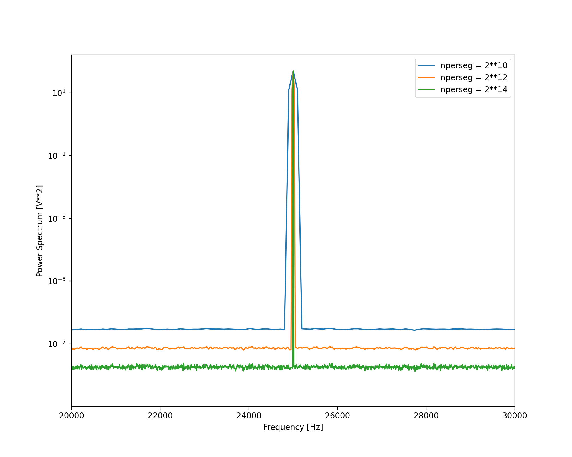
Figure 2: Power spectrum of a carrier with additive noise. Power spectrum is calculated with Welch method. The nperseg is changed between each plot.

To better illustrate the difference between spectrum and density, I’ve plotted three Welch spectrums, with different nperseg values. The nperseg value will control the frequency bandwidth of each frequency bin. Notice that the power of the carrier stays the same each time, but the total power of the noise changes. The total power of the noise across $[0, f_s/2]$ must stay the same. As nperseg is increased, the bandwidth of a frequency bin decreases, which means that there are more frequency bins across $[0, f_s/2]$. The total power, integrated across all frequency bins, is constant. So as the number of bins increases, the total noise power in each bin decreases.

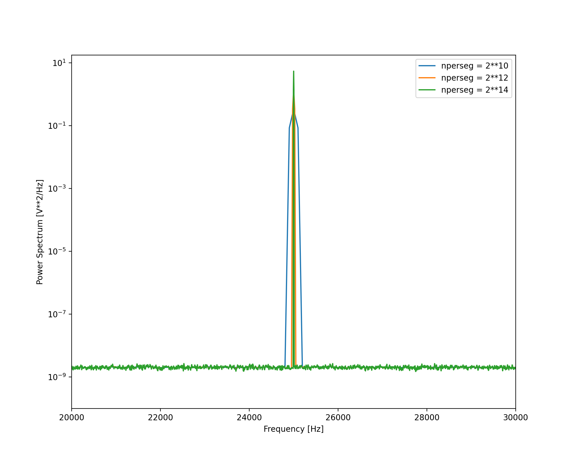
Figure 3: Power spectral density of a carrier with additive noise. Power spectral density is calculated with Welch method. The nperseg is changed between each plot.

Rather, if we were instead interested at looking at the additive noise, we should normalise the power spectrum to the resolution bandwidth of the bin. This is the power spectral density, which is obtained when passing density to the Welch method.

To extract the phase from this simulated signal, we can use SciPy’s signal.hilbert function, which provides the analytic signal.

analytic_signal = signal.hilbert(carrier)
instantaneous_phase = np.unwrap(np.angle(analytic_signal)) - 2*np.pi*fc*t

down_shifted = analytic_signal * np.exp(-1j*2*np.pi*fc*t) # down shift the analytic signal by fc
phase_down_shifted = np.angle(down_shifted)

We can choose to calculate the instantaneous phase of the signal, which is calculated with np.angle(analytic_signal), or we can first down shift the analytic signal and then calculate the phase. The instantaneous phase includes the frequency of the carrier, which should be removed. We can then calculate the phase PSD.

f1, Pxx1 = signal.welch(random_noise, fs, nperseg=nperseg)
f3, Pxx3 = signal.welch(phase_down_shifted, fs, nperseg=nperseg)
scaled_additive_noise_PSD = 2 * Pxx1 / A**2

plt.figure()
plt.plot(f1, Pxx1, label='Generated additive noise')
plt.plot(f1, scaled_additive_noise_PSD, label='Scaled additive noise')
plt.plot(f3, Pxx3, label='Phase from down shifted')
plt.axvline(x=fc, color='k', linestyle='--', label='Carrier frequency')
plt.legend()
plt.yscale('log')
plt.xscale('log')
plt.xlabel('Frequency [Hz]')
plt.ylabel('Power Spectrum [rad**2/Hz]')

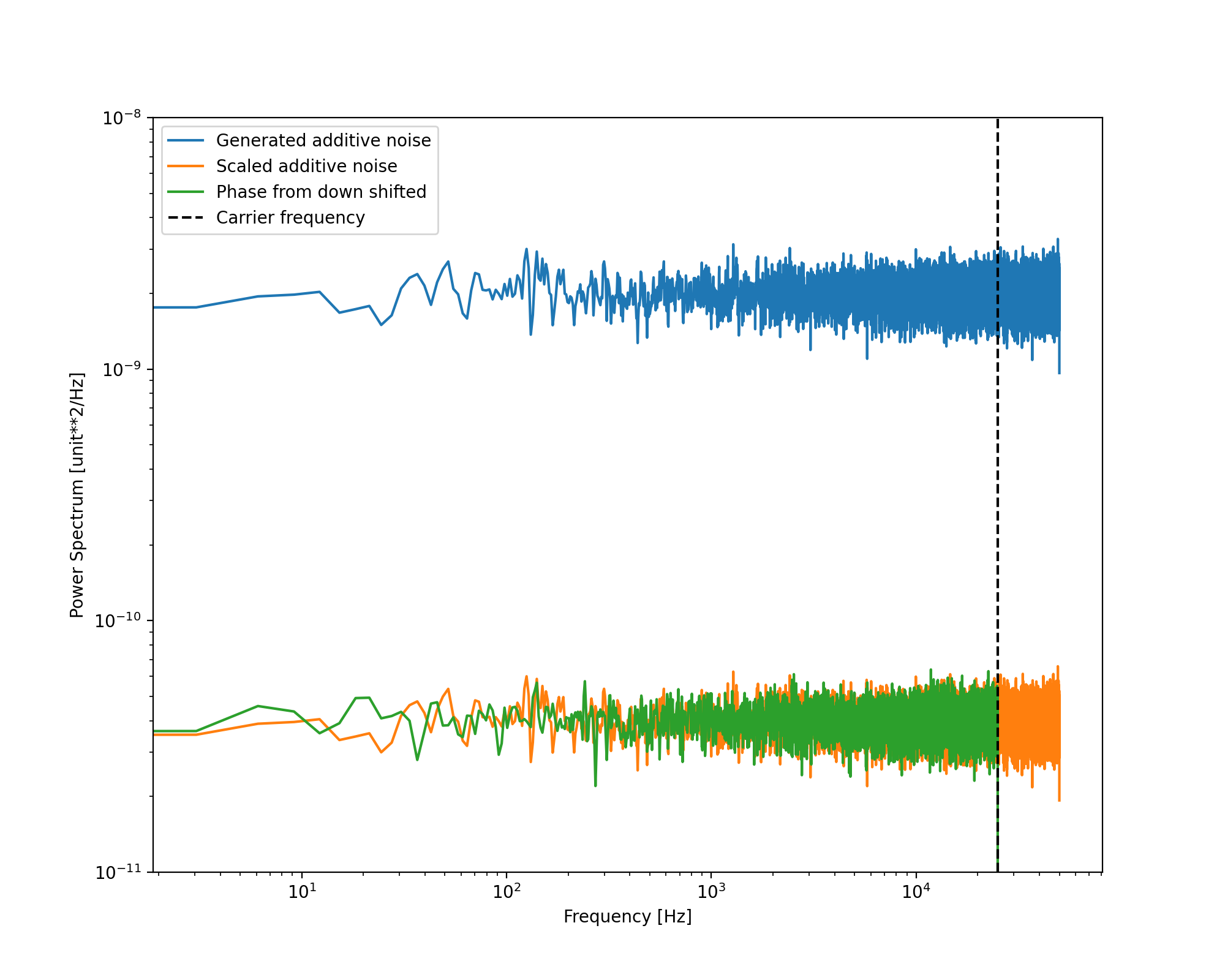
Figure 4: Phase power spectral density of generated additive noise, scaled additive noise and the calculated phase of the signal. Here, the PSD of the additive noise is an amplitude PSD, while the units of the scaled additive noise and the phase PSD are in radians.

Figure 4 shows the PSD of the generated additive noise, which would be in units of $V^2/\text{Hz}$, the scaled additive noise, obtained from $S_\phi(f)=S_{\bar A}(f)/A^2$ in units of $\text{rad}^2/\text{Hz}$, and the calculated phase also in units of $\text{rad}^2/\text{Hz}$. We can see that the additive to phase noise conversion holds for this choice of carrier frequency, amplitude and noise level. If we decrease the amplitude of the signal, we would expect the measured phase noise to increase. We can also see a cut-off at the carrier frequency, this won’t be a concern when we get to generating IQ samples. I’ve hidden the explanation for it, but it’s to do with the Fourier transform of the analytic signal.

Run this simulation locally, and play around with different parameters. Essentially, we’re simulating an arbitrary SNR, and investigating how it will limit our measurement of phase. A brief example is plotted in Figure 5.

test_modulation = 0.1 * np.sin(2*np.pi*100*t) # Simulate a phase modulation
A1 = 1 # strong SNR
A2 = 0.01 # weak SNR
carrier1 = A1*np.cos(2*np.pi*fc*t + test_modulation) + random_noise # same additive noise
carrier2 = A2*np.cos(2*np.pi*fc*t + test_modulation) + random_noise # same additive noise

analytic_signal1 = signal.hilbert(carrier1)
analytic_signal2 = signal.hilbert(carrier2)

down_shifted1 = np.angle(analytic_signal1 * np.exp(-1j*2*np.pi*fc*t))
down_shifted2 = np.angle(analytic_signal2 * np.exp(-1j*2*np.pi*fc*t))

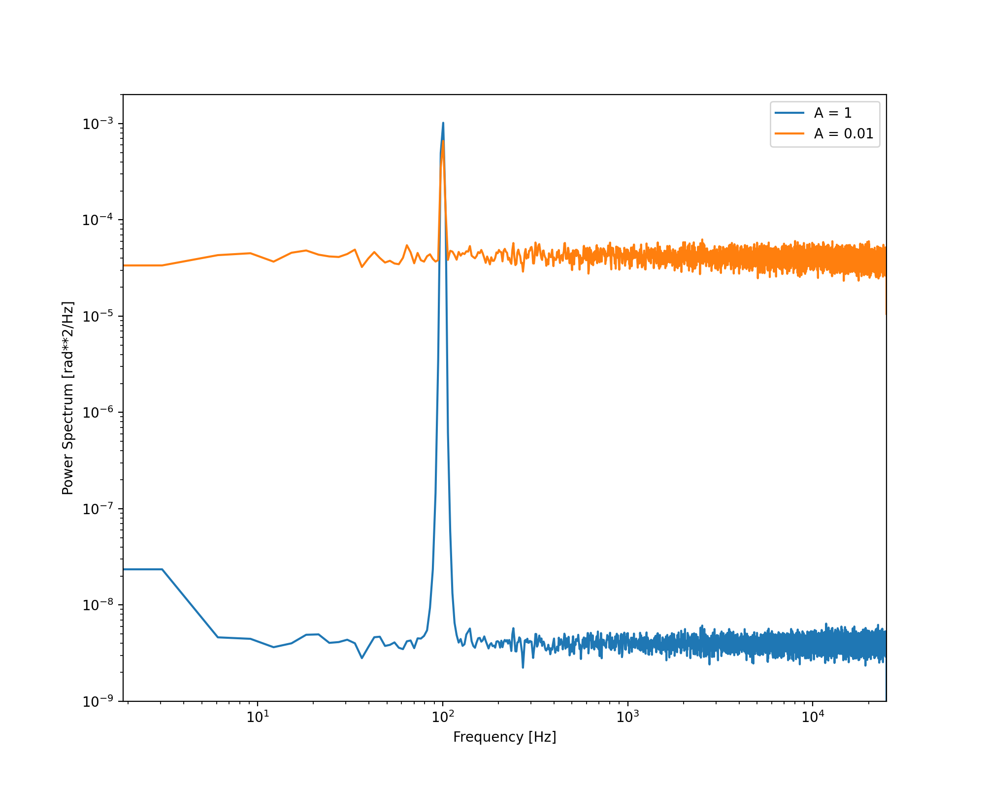
Figure 5: Phase power spectral density of a signal with a phase modulation. Here, the signal-to-noise (SNR) is adjusted by decreasing the simulated amplitude $A$.

Between each phase calculation, the additive noise is not changed. However, as the amplitude is decreased, the SNR between each phase calculation is much worse. We can start to see how additive noise can become an issue when tracking the phase of weak carriers. It’s also a good idea to take a look at the time-series, so we don’t get too lost in the PSD. The PSD is a tool to help us understand what’s happening in our time-series. Note that I’ve used different amplitude values, and a stronger phase modulation, as the NumPy np.unwrap() routine struggles to unwrap phase data with a lot of noise (a problem which will be addressed with the software PLL), and the stronger phase modulation is easier to visualise.

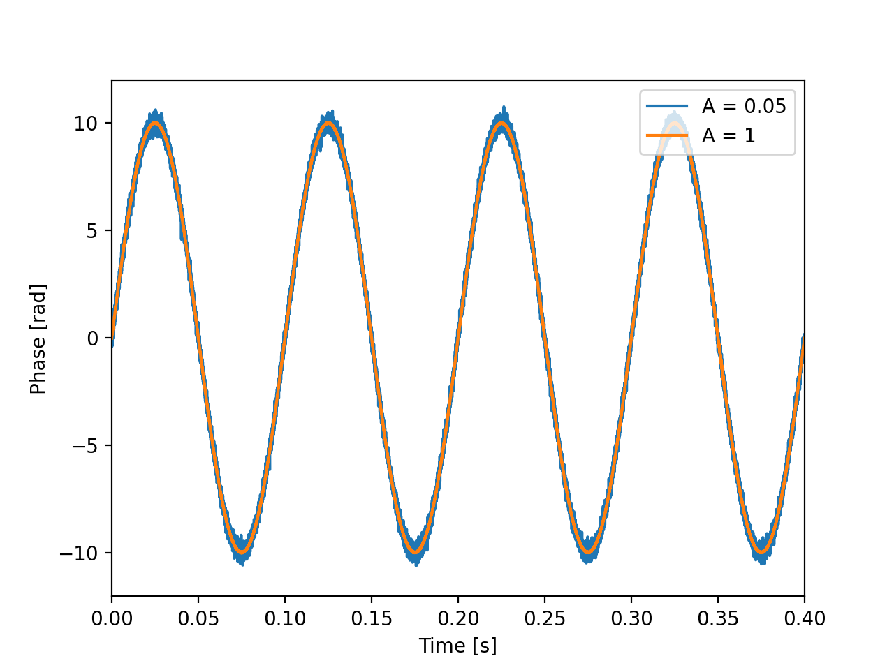
Figure 6: Phase time-series of a signal with a phase modulation. Here, the signal-to-noise (SNR) is adjusted by decreasing the simulated amplitude $A$.

References

[1] “PySDR: A Guide to SDR and DSP using Python.” [Online]. Available: https://pysdr.org/#

[2] E. Rubiola and F. Vernotte, “The Companion of Enrico’s Chart for Phase Noise and Two-Sample Variances,” IEEE Trans. Microwave Theory Techn., vol. 71, no. 7, pp. 2996–3025, Jul. 2023, doi: 10.1109/TMTT.2023.3238267.

[3] “hilbert — SciPy v1.15.2 Manual.” [Online]. Available: https://docs.scipy.org/doc/scipy/reference/generated/scipy.signal.hilbert.html

[4] Mathuranathan, “Understanding Analytic Signal and Hilbert Transform,” GaussianWaves. [Online]. Available: https://www.gaussianwaves.com/2017/04/analytic-signal-hilbert-transform-and-fft/

[5] “Effects of Additive Noise,” in Phaselock Techniques, John Wiley & Sons, Ltd, 2005, pp. 123–142. doi: 10.1002/0471732699.ch6.